A Bumpy Ride

Texas is a large, diversified state boasting the ninth largest economy in the world. At $2.4 trillion, its gross state product accounts for almost 10 percent of all economic activity in the U.S. In an economy of such size, it should be no surprise that parts of the state perform better than others. One example is the wide-ranging performance of industrial real estate in the state’s 25 Metropolitan Statistical Areas (MSAs) during the last 40 years.

While an earlier article, “Industrial Space Race: Texas Market Overview," showcased industrial market diversity in Austin, Dallas-Fort Worth, Houston, and San Antonio, this article considers the individual performance of all 25 MSAs. The goal is to assess changes in industrial inventory over the business cycle from 1982 to the close of 2022.

During the course of this study, two key findings emerged.

Find​​ing 1: Which Markets Diverged, and When

The motivating question for this research was whether the large markets began growing faster than the small markets around 2014. The short answer is that, in general, growth picked up across Texas, but the larger markets did exceptionally well compared with most small markets.

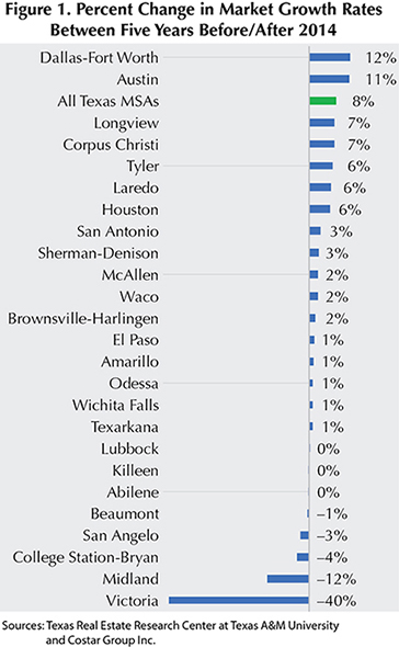
In the five years before fourth quarter 2014, the average growth rate across all metros was 4 percent. After 2014, the average increased to 12 percent. A closer look shows which markets were growing faster or slower than the average before and after 2014.

Before 4Q2014, small markets performed relatively well as a class, but some did better than others. Ten markets grew faster than the state average, and only two of them—San Antonio and Houston—were among the “Big Four." The five fastest-growing markets were all smaller metro areas: Victoria, Midland, San Angelo, College Station-Bryan, and Laredo. The top ten best performers averaged a 14 percent growth rate. The 15 markets that grew at a slower rate than the state average grew at only 1 percent.

As growth accelerated after 4Q2014, the big markets performed exceptionally well. The average growth rate across all 25 MSAs was 12 percent, but this growth was concentrated in fewer markets. Only five markets grew faster than the state average, and three of these—Dallas-Fort Worth, Austin, and Houston—were from the Big Four. The 20 markets that grew slower than the state average grew at 5 percent. Figure 1 shows how much growth rates increased or decreased in each MSA in the five years before and after 2014.

What about growth over the longer term?

Based on how they fared during the five national expansions and four recessions since 1982, individual markets tend to perform consistently. Markets that grow faster tend to grow faster throughout the business cycle. There is a 65 percent positive correlation between a market’s performance over expansions and recession periods.

Table 1 shows how markets ranked in terms of growth rates across the business cycle phases. For instance, Abilene’s average rank across all nine phases of the business cycle was 22^nd out of 25. It performed a little better during the five expansionary phases, ranking 19^th. It ranked 22^nd again during the four recessions. The top-ranked markets in terms of growth over all business cycle phases since 1982 were Laredo, Austin, San Antonio, Dallas-Fort Worth, and McAllen. See the data appendix for detailed growth statistics for all markets over each business cycle phase.

Finding 2. How T​​​exas Markets Clustered

When markets are grouped by their overall performance since 1982, a few geographic patterns emerge. These patterns can be defined by classifying markets in terms of whether they grew faster than the state average over each business cycle phase. Doing this shows some markets consistently grew faster than the average in all or most expansions and recessions, some consistently grew slower than average, and some had mixed results.

The three-by-three matrix in Figure 2 assigns each market to a cell. The columns define the number of expansions in which the market grew faster than average in expansions, and the rows define the same for recessions. The closer to the upper right, the better the MSA’s performance; the closer to the lower left, the worse the MSA’s performance. At first inspection, three groups of markets emerge.

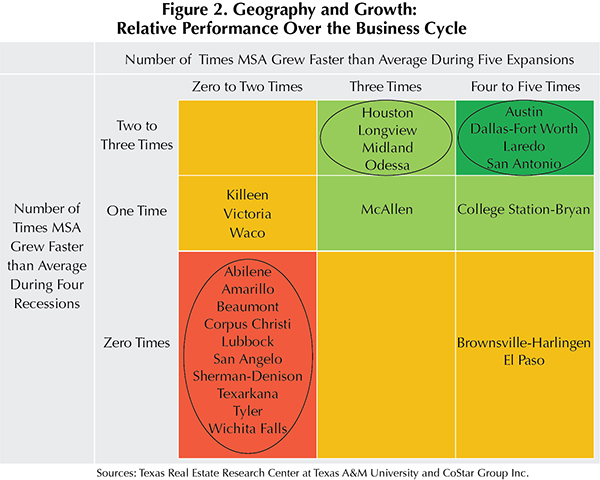
The top-tier performing markets—those that tended to grow continuously—are all along the I-35 corridor. A second tier includes mostly energy leaders that grew faster than the MSA average during most expansions and at least one recession. McAllen and College Station-Bryan also fall into this performance tier. A third cluster of poorer-performing markets include ten smaller metro areas that are mostly in West Texas or East Texas, outside the major growth corridors of the Texas Triangle. Other markets do not fall into these neat categories.

The apparent spatial clustering of markets in terms of inventory growth is not completely surprising. This raises more questions about local market differences and how they experience broader business cycles. Opportunities for future research include exploring how factors such as workforce skills and industry structure might explain the divergence and clustering of Texas industrial markets.

The term “business cycle" is a helpful shorthand for economic ups and downs over a long time.

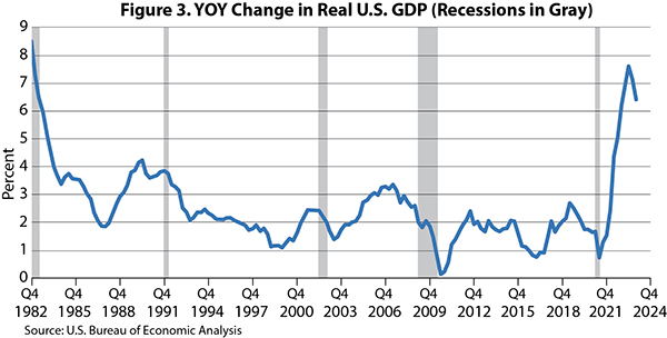
The broadest way of measuring the business cycle is with Gross Domestic Product (GDP). This statistic is calculated by the U.S. Bureau of Economic Analysis (BEA) for each calendar quarter. It is defined as the final dollar value of all goods and services sold in that quarter. Figure 3 plots the change in U.S. GDP since 1982 and indicates recessions with gray vertical bands.

While the BEA produces GDP estimates, it does not define the stages of the business cycle (Table 2). That role is assumed by a private entity with a government-sounding name: the National Bureau of Economic Research (NBER). A group of eight leading academic economists at NBER have identified what they consider to be the turning points in the U.S. economy since just before the American Civil War.

The NBER does not use the commonly assumed definition of a recession as two consecutive quarterly declines in GDP. In practice, they look at many economic indicators. Their careful deliberations take time, and the economy may be in a new phase before the last phase has been officially named. The U.S. economy could be in a recession now, but NBER may not declare a recession for some months.

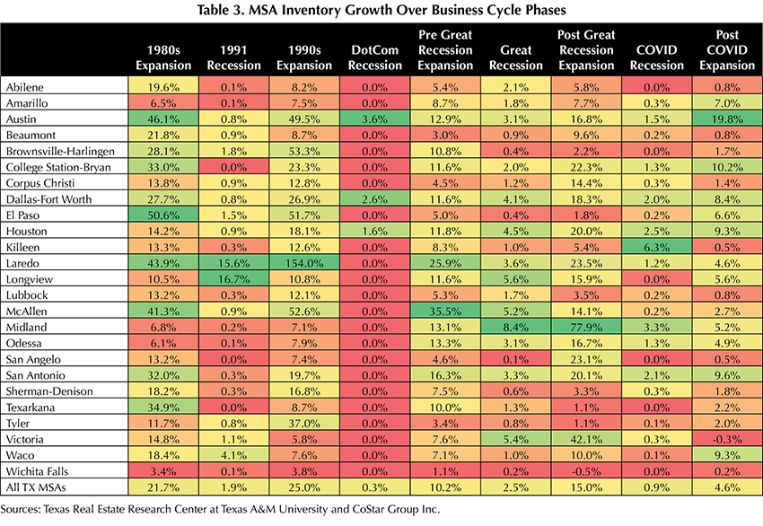
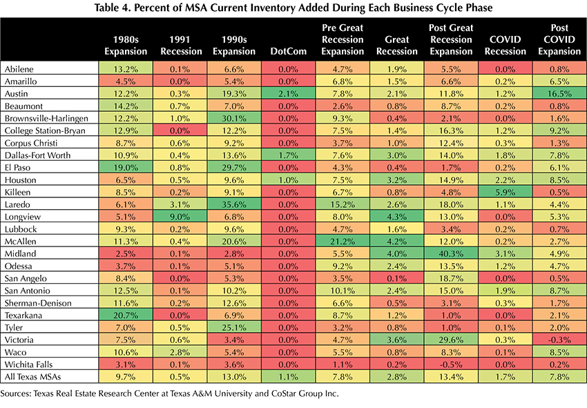
This data appendix presents inventory change details for all 25 Texas MSAs.

Table 3 shows total percent inventory change over each phase of the business cycle since 1982. Table 4 indicates what percent of current industrial inventory was delivered during each phase of the business cycle.

The color coding in each table classifies the metro areas’ performance within each phase. That is, the color coding changes in each column. Larger numbers are shaded green, smaller numbers are shaded red, and the average numbers are yellow.

____________________
Dr. Oney ([email protected]) is research director with the Texas Real Estate Research Center at Texas A&M University.